Agreeable Instantia

Welcome to the most recent installment of Agreeable Instantia! Agreeable Instantiations Volume 6: Definability and Computability in Algorithmic Information Theory

This week’s volume will center around the development of the concepts of definability and computability and their contribution to the foundation of Algorithmic Information Theory. Importantly, Definability and Computability and their formulation as established mathematical concepts help pave the way for a number of important mathematical results, conclusions and realizations. 

This week’s volume aims to discuss concepts of a particular kind of sharpness: objects that are perfectly well-defined yet provably beyond algorithmic reach. 

Kolmogorov complexity K(x) is specified as “the length of the shortest program that outputs x,” but there is no general procedure that computes K(x) from x. 

Chaitin’s halting probability $\Omega_{U}$ is specified as a weighted sum over halting programs for a universal prefix-free machine $U$, yet no algorithm can output its bits in full. 

Solomonoff induction, meanwhile, defines an ideal predictor by weighting over all programs, but that very universality prevents an exact solution from being computed; to know exactly how much weight to assign, one must know all programs which ever produce outputs consistent with the observed prefix.

As for Kolmogorov complexity, Chaitin’s halting probability and the Solomonoff induction prior, each of these quantities are uncomputable. With Chaitin’s halting probability and the Solomonoff prior, every single one of their digits are uncomputable, from the first to the last bit. As an integer quantity, Kolmogorov complexity is still uncomputable, but does not require an infinite amount of bits to exactly specify, like Chaitin’s constant and the Solmonoff prior.

In Algorithmic Information Theory, Definability is always logically and literally formulable, while Computability sometimes requires an exhaustive endurance often requiring more time and space than we have to fathom.

As one of the most important modes of both being and becoming, reading is both evidence of the existence of effective action and a reason for such existence. In computation, “reading” has a literal meaning. A machine reads a symbol, consults a rule, and takes the next step. Its run is nothing but a long chain of such readings—local interpretations accumulating into global behavior.

It has been written—by poets, philosophers, and religious minds alike—that “who runs may read,” a proverb about making a message so plain it can guide action even at full speed. Traditionally, it praises clarity: write the vision so plainly that even a hurried passer-by can grasp it. 

But in the computational setting the direction reverses. The program is the text, the machine is the runner, and what we want is not simply that the runner can read—but that we can consciously recognize what the runner is doing. We want an account of the run that amounts to understanding rather than mere notation: an accounting that not only describes but predicts, compresses, and explains.

Turing’s model makes the limits of that ambition precise.

Computation is embodied by what can be carried out mechanically, yet much of what we most want to extract from a computation—its long-run behavior, its minimal description, even whether it will ever stop—resists being simply “read off” from finite execution. 

Algorithmic information theory studies exactly this boundary: the space where definability remains within reach, while computation and meta-computation become exhaustive—or intractable.

As they pertain to the topics considered in this week’s volume, Definability and Computability belong to the arenas of mathematics, logic, and algorithmic design and evaluation (ie. computer programming)—and many of the examples we will consider in this week’s volume will involve the intersection of these fields of study. 

But first, before we are to discover the contents housed in this week’s volume, there are a number of important definitions to cover. 

Let’s start with definability; the definition of definability may seem to be an exercise in circular reasoning, but if we are careful to pay attention to the context(s) in which we aim to employ definability, a more nuanced understanding may emerge from the discussion. 

In mathematics and logic, Definability refers to whether a concept, object or set can be precisely described within a formal language or system. A canonical example is the set of even numbers being definable in first-order logic using arithmetic. 

In algorithmic information theory, “definability” is often treated as describability: an object is specified by a program for a universal machine, and the central question becomes how short the best such description can be.

AIT considers description length (Kolmogorov complexity) to measure how much information is needed to specify/produce an object —and the bounds of what can and/or can’t be computed about that requirement.

Computability, as defined by Alan Turing, involves the existence of a Turing machine that, when given n, halts with output f(n). 

So, what is a Turing machine and how does it work?

A Turing machine is a theoretical model of computation introduced by Alan Turing in 1936. It is a mathematical abstraction that captures the fundamental principles of algorithmic computation and forms the basis for modern computer science.

Components of a Turing Machine:

A Turing machine consists of:

1. An infinite tape divided into discrete cells (like memory), each holding a symbol from a finite alphabet.
2. A tape head that:
   • Can read the symbol at the current tape cell.
   • Can write a new symbol.
   • Can move left or right by one cell.
3. A finite set of states (including a start state and one or more halting states).
4. A transition function that:
   • Determines what to do based on the current state and symbol read.
   • Specifies the next state, what symbol to write, and which direction to move.

How Does a Turing Machine Work?

1. The machine begins in a start state with its head at a particular location on the tape.
2. It reads the symbol under the tape head.
3. Based on the current state and symbol, it:
   • Writes a new symbol,
   • Moves left or right,
   • Transitions to a new state.
4. This process repeats until the machine enters a halting state (if ever), at which point it stops.

A halting Turing machine is one that eventually reaches a halting state and stops after performing a finite number of steps on a given input.

• Whether a Turing machine halts depends on both the program (transition rules) and the input.
• The Halting Problem (Turing, 1936) shows that there is no general algorithm that can determine whether an arbitrary Turing machine will halt on an arbitrary input.

In programming, Computability describes what functions you can write an algorithm for—where the algorithm is guaranteed to eventually give a correct result. For example, computing factorials is computable, while a general algorithm for deciding whether any arbitrary Turing machine halts is not computable due to the well known halting problem. 

Definability and Computability by themselves have many applications in math, logic and computer science, but the introduction of another concept will lay the foundation for an important branch of mathematics known as Algorithmic Information Theory—Kolmogorov complexity.

The Kolomogorov Complexity K(x) of a string x is the length of the shortest program that generates x on a universal Turing machine. 

In fact, according to the strict definitions of definability and computability we considered above, Kolmogorov complexity is definable, but uncomputable. 

Furthermore, Kolmogorov Complexity provides the foundation for a strict mathematical and logical definition of randomness. A string x is algorithmically random (known as Martin-Löf random) if K(x) ~ |x|. In other words, if a string is Martin-Löf random, the shortest program producing x is essentially the same length as x. 

Kolmogorov complexity is uncomputable because there is no general algorithm for computing K(x) given any string x. However upper bounds can always be computed for specific strings, once we restrict our attention to a chosen string or set of strings. 

For example, a string of one million zero’s 0000….00000, can be algorithmically described as “Print 0 one million times”. 

Advancements made by Kolmogorov, Solomonoff and Chaitin in the field of Algorithmic Information Theory capture many of the concepts described above and also help reframe Godel’s interrogation of mathematical incompleteness as a quantitative one. 

In Algorithmic Information Theory, the absence of provability of certain statements within formal logical systems described by Godel’s First Incompleteness Theorem is effectively translated to an absence of algorithmic computability.

Tracing the development of Algorithmic Information Theory, many results point to the form of important consequential facts relevant to the field. 

First, the formal definition of randomness makes it a mathematical property, not just a statistical one. 

Also, compression is recognized as a form of tractable understanding: a compressible string contains non-randomness, in the sense that it admits a substantially shorter effective description than itself. K(x) can be much smaller than $|x|$ (highly structured/regular) or close to $|x|$ (incompressible/random). While no general method exists for finding the minimal description length K(x) for an arbitrary input x, we can still obtain informative upper bounds by restricting attention to a fixed model class (or by using practical compressors). Within such restricted settings—and for the kinds of structure those models are designed to detect—we can often estimate compressibility quite well.

Furthermore, uncomputability shapes the limits of prediction: there is no single algorithm that can solve every instance of these general model-selection and prediction tasks. As the No Free Lunch Theorem tells us, inductive bias is the price we pay for algorithmic specification. What we should hope for are computations that are optimal within a restricted context and hypothesis class, and we should expect performance to degrade—sometimes sharply—when an algorithm of a restricted class is taken out of its natural habitat.

Finally, formal systems cannot capture all truth: because arithmetic truth is not definable within arithmetic (Tarski), no sound, computably axiomatized theory can be complete. In AIT this becomes quantitative: any fixed theory can determine only finitely many high-complexity facts (Chaitin), such as only finitely many bits of Ω, and even when we have computed finitely many bits of Ω, we have no way of knowing how many of these bits are exactly correct.

The quantitative instantiation of Godel’s incompleteness hinted at above is perhaps best given by a concept introduced to AIT by Gregory Chaitin. Aptly named Chaitin’s constant, Chaitin’s Ω is defined as the halting probability for a universal prefix-free Turing machine. In layman’s terms, Chaitin’s constant is the probability that a randomly generated program will halt. 

Without giving a total explanation, randomly generating programs is more difficult than initially thought. Both mechanically and notationally. Any arbitrary bit string cannot be considered as a valid program because one program can be the prefix of another—the machine would have no way of knowing when one program stops and another program starts. 

Thus Chaitin’s constant focuses its attention on prefix-free (self-delimiting) codes, which is the set containing all bit-strings which are not prefixes of any other.

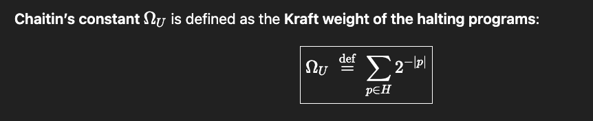
Fix a universal prefix-free machine $U$. Its transition function is the fixed “interpreter,” and each finite bit-string $p$ on the input tape is a candidate program. Because the set of valid programs is prefix-free, the weights $2^{-|p|}$ satisfy Kraft’s inequality. Chaitin’s halting probability is then

$$\Omega_U \;=\; \sum_{p:\,U(p)\ \text{halts}} 2^{-|p|},$$

the total measure of the halting domain of $U$. Crucially, $\Omega_U$ depends only on whether programs halt, not on whether their outputs meet any external “goal”—and its binary expansion encodes halting information in a maximally compressed way.

For the standard definition, there is one halting probability $\Omega_U$​ for each chosen universal prefix-free machine $U$, and the only property being counted is halting:

This dependence on the choice of $U$ is not a flaw but a feature. Any realization of Chaitin’s constant is associated with a specific universal prefix-free machine, and a different choice typically yields a different value. Notationally:

$$U \neq U’ \quad \Longrightarrow \quad \Omega_U \neq \Omega_{U’}.$$

Chaitin’s constant does not compute a particular target output or function; rather, it measures the total Kraft-weighted mass of programs that eventually halt on $U$—equivalently, the probability that a randomly generated self-delimiting program halts when run on $U$. The machine $U$ must be universal (able to simulate any other machine given a suitable program) and prefix-free (self-delimiting, so programs form a prefix code), and it must have a designated halting condition so the event “halts” is well-defined.

The depth of $\Omega_U$​ is that it compresses halting information into a single real number: knowing the first $n$ bits of $\Omega_U$​ is enough (up to machine-dependent constants) to determine which programs of length $\le n$ halt. This is why $\Omega_U$​ functions as a compressed ledger of halting facts—and why, for universal prefix-free $U$, $\Omega_U$​ is algorithmically random (Martin-Löf random) and also why its binary expansion behaves as an algorithmically random sequence.

The exact first $n$ bits inevitably carry about $n$ bits of irreducible and uncomputable information, once your running partial sum of discovered halting weights is within $2^{-n}$ of Ω, no additional length ≤ n halting programs can remain undiscovered if this truly the first n bits of $\Omega_U$​ —otherwise the sum would jump by at least $2^{-n}$ and overshoot the interval.

But crucially, while the partial sums are always safe lower bounds, there is in general no computable way to know that we have entered the correct $2^{-n}$-interval: that missing piece is the first hint of Ω’s one-sided (left) semi-computability.

What we can do is accumulate better lower bounds; what we cannot do uniformly is estimate how far we are from the truth—an asymmetry that will later reappear as ‘left- vs right-semi-computability.

More formally, Chaitin’s argument shows that if $K(\Omega_U{\upharpoonright}n)$ were much less than n, then you could build a paradoxical compression: the “too-short” description of $\Omega_U{\upharpoonright}n$ would allow constructing a short program that produces something it shouldn’t be able to, thus an absurdly short description yielding halting information for programs up to length ≤ n.

This yields the incompressibility bound

$$K(\Omega_U{\upharpoonright}n)\ \ge\ n – O(1),$$

which is exactly the criterion for Martin-Löf randomness.

Furthermore, in his book Meta-Math (https://arxiv.org/pdf/math/0404335), Chaitin shows that randomness and incompleteness leak all the way down into arithmetic: there are explicit Diophantine equations whose pattern of solvability—sometimes phrased as existence of solutions, and in some constructions as finitude versus infinitude of solutions—encodes the bits of Ω. In that sense, deciding or proving those algebraic facts would amount to extracting halting information: if an effective method could settle the relevant solvability questions uniformly, it would thereby decide instances of the halting problem.

In fact, the MRDP theorem (Matiyasevich–Robinson–Davis–Putnam) resolved Hilbert’s tenth problem in 1970 by proving that no general algorithm exists to determine if an arbitrary Diophantine equation (polynomial with integer coefficients) has integer solutions via its equivalence to determining if a Turing machine halts, which is undecidable. 

In this volume, K(x) denotes prefix Kolmogorov complexity, so that K$_U$(x) and $\Omega_U$​ are defined relative to the same universal prefix-free Turing machine framework.

Prefix Kolmogorov complexity has an algebraic shadow of its own. Fix a universal prefix-free machine $U$. The relation $K_U(x)\le n$ is computably enumerable: we can dovetail-run all programs of length at most $n$, and whenever one halts with output x, we eventually discover it. By the MRDP, any c.e. relation can be written as “there exists integers $\vec y$ such that a polynomial equation holds.” So there is a polynomial $P$ with integer coefficients such that:

$$K_U(x)\le n \quad \Longleftrightarrow \quad \exists \vec y\in \mathbb{Z}^m\; P(x,n,\vec y)=0.$$

The complementary statement is fundamentally harder: a lower bound like $K_U(x)>n$ is not c.e. in general, so it does not come with the same “witness” Diophantine encoding. Deciding that no shorter program works would require precisely the negative halting information computation cannot generally provide—another preview of the asymmetry between what we can bound from below and what we can bound from above.

There is an interesting place where the halting problem reappears wearing algebraic clothing. MRDP tells us that no general method can decide, for every polynomial equation, whether it has an integer solution. In a later volume we will follow this thread: how computation casts an algebraic shadow, how Ω can be encoded into Diophantine families, and why the obstruction is once again the impossibility of proving universal negatives —especially when “has not yet halted” is never the same as “will never halt.”

Solomonoff induction, on the other hand, involves a uniquely brave method to optimally predict the next character after observing a sequence x. 

$$M(x)=\sum_{p:\,U(p)\ \text{outputs a string with prefix }x}2^{-|p|}$$

Formally, Solomonoff’s universal prior $M(x)$ is an Ω-like Kraft-weighted sum, but over the occurrence of the output beginning with $x$, rather than the occurrence of the computation halting.

By leveraging a weighted partial Kraft sum over all programs that output a string with the prefix being x, the Solomonoff prior computes an optimal prediction algorithm over all programs of length n when computed to n bits. 

And like Kolomogorov complexity and Chaitin’s constant, the Solomonoff prior is definable but uncomputable. 

As with the cases of uncomputability considered in this week’s volume, the prediction problem as posed by the Solomonoff prior is uncomputable. Furthermore, like Chaitin’s constant, the Solomonoff prior is uncomputable yet also left semi-computable, meaning there is no general procedure that outputs it exactly or provides computable error bounds.

However there are classes of prediction problems that are solvable with computation. One such instance is Universal Prediction: it assumes the data are generated by some process inside a chosen hypothesis class, and it competes with the best predictor in that class by minimizing cumulative log loss. Concretely, we fix an allowable family of stochastic models—often something like i.i.d., finite-order Markov chains, or more generally a parametric/ergodic class—and treat each model as a probability distribution over strings.

Universal prediction then forms predictions by (explicitly or implicitly) performing Bayesian model averaging over that family (or equivalently, choosing a code that is optimal for that family), so that its log-loss is asymptotically as small as if we had known the best model in advance. In this setting, “optimal prediction” and “optimal compression” coincide: minimizing expected log-loss matches minimizing codelength, so universal prediction is tightly linked to universal coding and the Minimum Description Length (MDL) principle. 

The Solomonoff prior seeks to perform a similar algorithmic optimization, however the hypothesis class of algorithms is all programs, and thus prohibits an exhaustive search yielding a global optimum. 

True story: As an undergraduate at MIT, I once received a final grade of Incomplete in a Graduate course in Inference and Information, for electing not to answer the final question on the final exam asking for a proof of the existence and effectiveness of Universal Prediction. Back then, I suppose I did not have a full mastery of the concept or an understanding of the full landscape. But I did enjoy the final project in which I wrote an algorithm to decrypt an encrypted text from its given cipher-text and also showed the algorithm to be a specific example of the algorithmic optimization paradigm known as Expectation-Maximization. 

Anyhow, here I will show that the Algorithmic Information Theoretic concern with Definability and Computability can help frame both the Solomonoff prior and Universal Prediction.

Consider the real numbers, any number between positive and negative infinity contains, no doubt, an uncountable amount of information. Furthermore, most of these numbers require an infinite amount of precision to describe. As noted by Chaitin in his book Meta-Math (https://arxiv.org/pdf/math/0404335), the measure of the set of all reals that can be individually named, specified, or even defined, constructively or not, within a formal language or individual Formal Axiomatic System has probability zero.

What we find here is that reals are undefinable with probability one. 

There are an uncountable number of real numbers and only a countable number of finite descriptions, thus the undefinable reals determine that the reals are undefinable with probability one. 

Still, even if we restrict our attention to definable reals, we should develop a quantitative and qualitative respect for the difficulty of computation—and for the difference between statistical unpredictability and algorithmic incomputability.

Consider that π is definable and computable: there exists an effective procedure that outputs its digits, and there are algorithms that approximate π with explicit, shrinking error bounds. Yet the digit sequence of π can still look “random” to restricted statistical models. A finite-order Markov predictor, such as one computed via Universal Prediction, for example, has no principled way to exploit the arithmetic structure of π; if π behaves like a normal number, as widely supported by statistical tests for randomness (https://arxiv.org/pdf/1612.00489) on trillions of its digits, then local frequency statistics won’t yield systematic advantage in predicting the next digit.

Solomonoff induction changes the picture precisely because it is not restricted to such local statistical mechanisms. By mixing over all programs, it assigns weight to the program(s) that compute π, and in that sense it can in principle learn to predict the successive digits of π: the computable structure is available to be discovered because it lies within the hypothesis class.

To take things a step further, consider that Chaitin’s Ω is definable but uncomputable. Fix a particular universal prefix-free machine $U$, and $\Omega_U$​ is a perfectly precise mathematical object—yet its successive bits encode halting information. Here both restricted statistical predictors and universal methods collide with the same barrier: there is no computable procedure that can predict the bits of Ω beyond what is already computably implied (and only left semi-computably), because doing so would amount to deciding halting cases.

A final distinction makes the theme concrete: left and right computability. Some uncomputable quantities are still approachable from one side. A real number is left-computable (lower semi-computable) if there is an effective process that produces an increasing sequence of rationals converging to it; it is right-computable (upper semi-computable) if there is an effective process that produces a decreasing sequence converging to it. These notions matter because they determine what kinds of error bounds computation can ever hope to consider. If a quantity is computable, we can approximate it to within any ε (approaching from above or below via left computation or right computation) and know we have done so; but if a quantity is only left-computable, we can keep producing better lower bounds without any general way to estimate how far we remain from the truth—no computable stopping rule yields a guaranteed margin of error. 

This is exactly where Chaitin’s Ω becomes a perfect object lesson. Ω is lower semi-computable because each time we discover a new halting program we can safely add its weight and raise a lower bound; but it is not upper semi-computable because tightening an upper bound would require the exclusion of programs which will never halt—precisely the negative information that computation cannot generally provide.

The lower bound can always rise for two reasons: programs we’ve already begun running in previous time trials may halt later, and programs we haven’t yet explored in future time trials—especially longer ones—may also halt and contribute additional weight. Exactly computing $n$ correct bits would require bounding the total remaining halting mass below $2^{-n}$, which demands negative information about which programs will never halt (and how much halting mass remains in the trailing digits).

K(x) is upper semi-computable because it asks for a minimum over programs, to arrive at a final answer, you would need to exclude all shorter candidates.

With the left computability of Ω and the right computability of K(x), in both cases the missing ingredient is reliable negative information: proofs that exclude certain programs which will never halt and/or will never produce x. The asymmetry comes from the same source: computation is good at accumulating positive evidence (a program halts; a program outputs x), and bad at verifying universal negatives (no shorter program works/halts; no unseen/shorter program will ever halt).

To be even more rigorous, $\Omega$ is algorithmically random (Martin-Löf random): its first $n$ bits are incompressible up to an additive constant, and no computable procedure can systematically predict or really even compute them. In this sense $\Omega$ is predictively hostile—not because it lacks information, but because it concentrates halting information in a form that resists any effective method of compression, extraction or verification.

By contrast, numbers like π are computable in the full two-sided sense: there are algorithms that deliver approximations together with provable, shrinking error bounds, making prediction and verification tractable; it is not merely estimable, but guarantee-ably so, and that is why prediction for π is a matter of computation while prediction for Ω is lost without any computable margin of error and would amount to require solving the halting problem itself.

In this contrast, “prediction difficulty” becomes precise: some targets, like π, admit convergent estimates with strict error bounds effectively ruling out errant values for a well informed prediction algorithm, while others—like Ω—admit only one-sided approximation and therefore frustrate any idea of exact computation, much less prediction.

This distinction also clarifies a sobering fact about the real line. Algebraic reals are countable and have measure 0. Computable reals—including π—are also countable and have measure 0. Even the set of definable reals (those singled out by any finite description in a fixed language) is countable, hence measure 0. By contrast, the set of undefinable reals is uncountable and has measure 1; and since every algebraic real is definable, every undefinable real must be transcendental. In this sense, “almost every” real number lies beyond both computation and definition.

Our varied choice of computation targets is made out of a respect for the measure of real number line. When undertaking computation it should be important to consider what sequence of digits are intended to be output and what kind of real number this constitutes. Many real numbers are computable, but in fact, most real numbers are not.

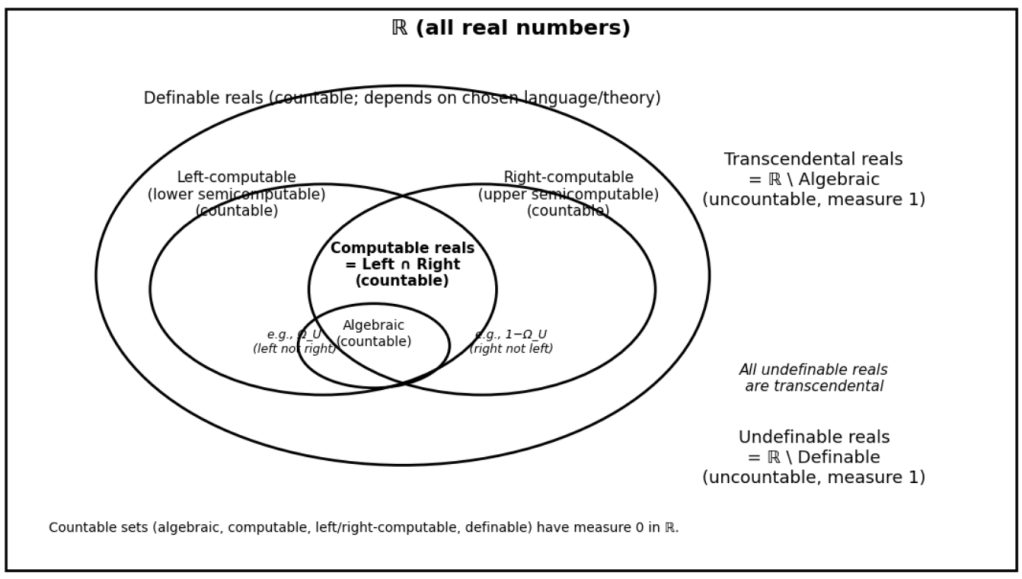
Under the standard first-order (parameter-free) notion of definability: algebraic ⊂ computable ⊂ definable, definable reals can be algebraic or transcendental and can be computable or uncomputable, and undefinable ⊂ transcendental while transcendental ⊄ undefinable.

Definability encourages the notion that computer programs mean what they say and say what they mean

Computability formalizes the necessity— and the difficulty —of the verification that computer programs mean what they do and do what they mean

As with many important undertakings in the universe, knowing what is right, and how right it is—is easier said than done

Ralph Waldo Emerson once remarked that “Permanence is a word of degrees”

Algorithmic Information Theory teaches us that definability may give permanence a name, but computing the global optima implied and required by such permanence is ultimately prohibited by the traditional limits of computation itself— constraints on time and memory.